
Point clouds: reading, clipping and thinning
Upload LAS, LAZ, E57, PLY or XYZ/PTS, see what is in it, and cut it down to the part you care about.
5 min read
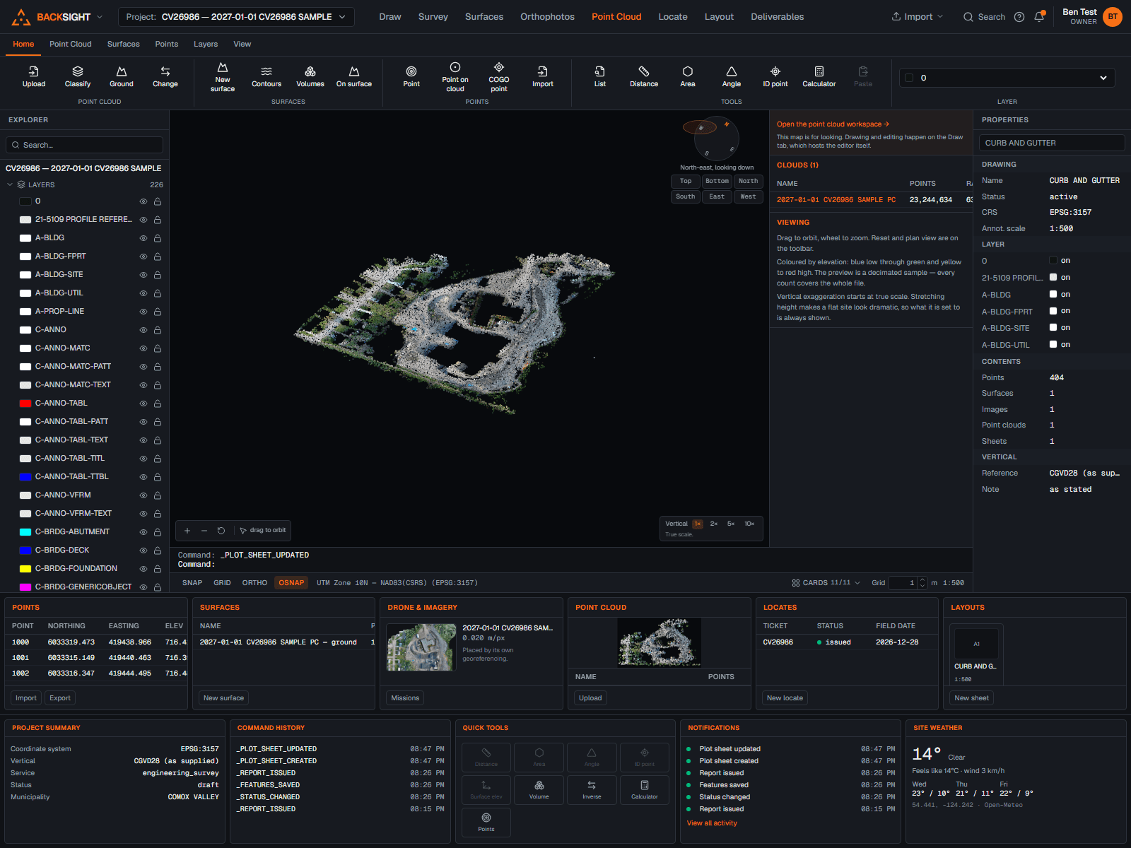
Uploading
- Import (top bar, any mode) → Point cloud, or Point Cloud mode directly, and upload a LAS, LAZ, E57, PLY or XYZ/PTS file.
- Name it, and state the coordinate system and vertical reference it is on.
- Backsight reads the header and reports the point count, the extent, and what classifications the file carries.
Note
A CRS declared inside the file is reported for you to confirm, never adopted silently. Clouds are never reprojected and their heights are never converted.
Anything that is not LAS is converted to LAS on the way in, so the reader, the ground classifier, the thinning and the surfaces all behave the same whatever the scanner wrote. Coordinates carry across to the millimetre and the panel says what the file arrived as.
What each format brings with it:
- E57, every scan in the file is combined, and each is moved by its own pose. A scan read without its pose sits where the instrument stood rather than where the site is. Returns the scanner flagged invalid are dropped and counted.
- PLY, ASCII or binary, either byte order. A classification is read when the file carries one; most exporters write none, and then every point is class 0 (never classified) and you can run the ground classifier yourself.
- XYZ and PTS, plain text, X Y Z on each line, separated by spaces, tabs or commas. A PTS point-count first line is recognised and skipped. Columns past the third are not imported.
Text files state no units and no coordinate system
An XYZ or PTS file carries nothing but numbers. The coordinate system and vertical reference you choose are taken at your word, and the numbers are used exactly as written, so check the file is in metres on the grid you think it is before you build anything from it.
Looking at it
- Colour by elevation, by classification, ground, vegetation and buildings told apart at a glance, or by the point's own colour when the file carries RGB, the way a drone cloud does. Both the colour and the density you settle on are saved with the cloud and used by every view of it: its own viewer, the Point Cloud tab, and the Draw tab's reference dots.
- Dot size, fine through heavy, is saved with the cloud too, so the same cloud reads the same way on the Draw canvas and in its own viewer.
- The viewer draws a decimated sample and says exactly how many of how many points it is showing. The Density control turns the sample up on demand, to half a million points, or every point when the whole cloud fits under that, re-read from the stored file each time.
- Densify this view re-samples inside exactly what is on screen, so density goes where you are looking. Zoomed in far enough that the view holds fewer points than the cap, you are seeing every single point there, and the label says so.
- Choosing a density reads the cloud once and keeps that sample as a file, so every later visit downloads it instead of re-reading the original, the same reason an orthophoto appears instantly the second time. Densify this view is situational and deliberately changes nothing that was saved.
- The classifications panel counts every class over the whole file, not just the sample.
- On the Draw canvas the cloud shows as reference dots, and the Point on cloud tool copies any dot into a real point, its exact coordinates and elevation, no surface needed first. Every sampled dot is an actual measured point from the file.
Making a smaller cloud
Clip and thin writes a new dataset and leaves the original alone.
- Draw a boundary on the view, if you want to clip to an area.
- Choose which classifications to keep, if you want only some.
- Set a keep-every-nth if you want it thinner.
- Derive. The new cloud records where it came from and what was done to it.
Tip
Every kept point travels byte for byte, thinning a cloud does not round anybody's coordinates.
Deleting points you can see
On the viewer, Select lets you pick points by clicking them, dragging a box, or drawing freehand around them, then Delete selected. What that does is write a new cloud without those points, the file you uploaded is the record of what was measured and is never edited, and the new cloud records which areas were removed and which cloud it came from. The count on screen is of the sample you are looking at; the delete applies to every point in those areas across the whole file.
Comparing two visits
Build a ground surface from each visit, then open Change detection on either cloud. Find changed regions lists every place that gained or lost more than your threshold, each pile and each cut on its own, with its area, volume, deepest change and centre, and Whole-site gained / lost gives the one number for the period. Both are measured exactly on the overlaid triangulations.
Give a region a name, Pile 3, North cut, in the Name column; it is saved beside the run and used wherever that region is mentioned. Every run is kept in the project's history, so a month's comparisons read back as a list, and Progress by region follows each region of the latest run back through the periods it stands on, with each period's own change. When a region in this period stands inside a region from the previous one, the previous run being the one whose later surface is this run's earlier, the table says so, with that region's volume and date. That is a statement about where it sits, not a claim that it is the same material.
Classify the ground first
Build both surfaces from ground points, by the file's own classification or by classifying here with the same settings for both visits. Trees, water and equipment that differ between flights are otherwise reported as change.
Read next
- Ground classification: keeping the file's, or classifying it hereThree ways to get ground points out of a cloud, what the classifier actually does, and how to set it.
- Building a surfaceTriangulate points into ground you can contour, measure and stake from.
- Volumes: against a datum and between two surfacesExact prismatic volumes, with the method and the area stated so the number can be checked.
Something here wrong or missing? Tell us and we will fix it.